External Graphics with knitr

This is part three of our four part series

• Part 1: Specifying the correct figure dimension in {knitr}.
• Part 2: What image format should you use for graphics.
• Part 3: Including external graphics in your document (this post).
• Part 4: Setting default {knitr} options.

In this third post, we’ll look at including eternal images, such as figures and logos in HTML documents. This is relevant for all R markdown files, including fancy things like {bookdown}, {distill} and {pkgdown}. The main difference with the images discussed in this post, is that the image isn’t generated by R. Instead, we’re thinking of something like a photograph. When including an image in your web-page, the two key points are

• What size is your image?
• What’s the size of your HTML/CSS container on your web-page?

Sizing your image

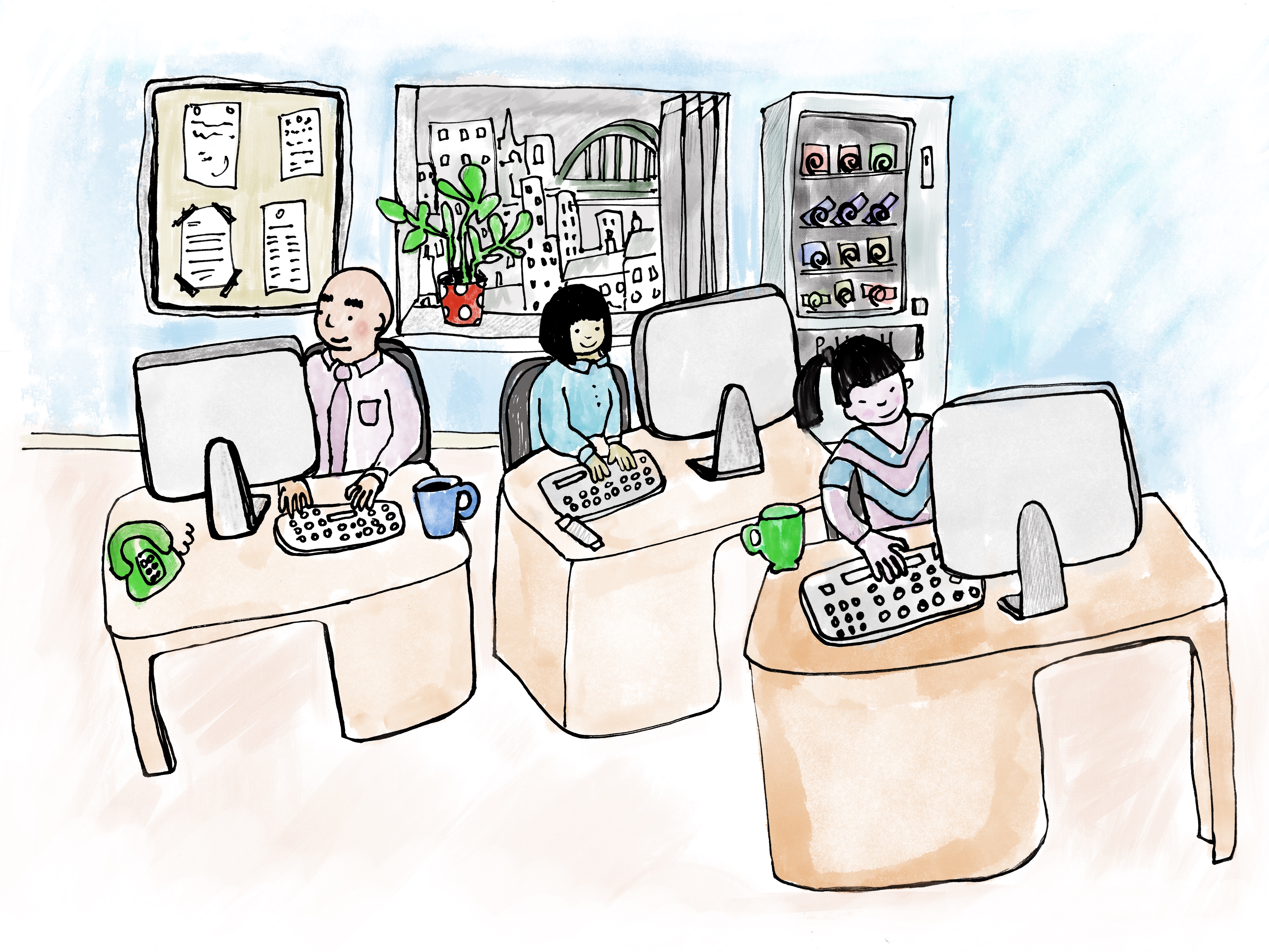
Let’s suppose we want to include a (pre-covid) picture of the Jumping Rivers team. If you click on the original picture, you’ll see that it takes a second to load and also fills the page. This is a very strong hint that the dimensions need to be changed. On our web-page, we intend to place the image as a featured image (think the header image of a blog post). The dimensions of this is 400px by 400px (typically the resolution will be larger than this).

We can determine the image dimensions of our original image using the {imager} package

library("imager")
original = imager::load.image("office.jpeg")
d = dim(original)[1:2]
d
#> [1] 4409 3307

As you might have guessed, the dimensions are far larger than required, 4409px by 3307px instead of 400px square. This, in turn, corresponds to an overly large file size

fs::file_info("office.jpeg")$size
#> 3.4M

My general rule of thumb, is

don’t lose sleep about images less than 200kb

Also, as the original image isn’t square, we can’t just squash the image into a square box, as this will distort the picture.

Instead, we’ll scale one dimension to match 400px

scale = max(d / 400)
img = imager::resize(original, 
                     imager::width(original) / scale, 
                     imager::height(original) / scale,
                     interpolation_type = 6)
img
#> Image. Width: 399 pix Height: 300 pix Depth: 1 Colour channels: 3

then pad the other dimension with a white background

square_img = imager::pad(img, 
                         nPix = 400 - height(img), 
                         axes = "y", 
                         val = "white")
imager::save.image(square_img, file = "office_square.jpeg")
square_img
#> Image. Width: 399 pix Height: 400 pix Depth: 1 Colour channels: 3

As we have scaled the image to have the correct dimensions, the file size is also smaller

fs::file_info("office_square.jpeg")$size
#> 24.4K

Including images in an R markdown File

We can include an image using {knitr} and the include_graphics() function, e.g.

knitr::include_graphics("office_square.jpeg")

Typically the chunk would use echo = FALSE as we don’t want to see the actual R code. As the image isn’t being generated by R, the chunk arguments fig.width and fig.height are redundant here - these arguments only affect graphics that are generated by R.

There are four core arguments for manipulating how and where the image is specified

• fig.align. Default left. In this page, I’ve set that to center.
• output.width & output.height control the output width / height, in pixels or percentages. The % refers to the percent of the HTML container.
• fig.retina takes a value 1 or 2, with the default being 2 (discussed below)

The arguments to control the output width / height are output.width / output.height, which accept sizes as pixels or percentages, using the string % or px as a suffix. The % refers to the percent of the HTML container. The crucial thing to note is that we if we size the width & height smaller than the actual image, then the browser will scale the image, but image will still be the same size, potentially impacting page speeds.

Setting out.width="200px" and fig.retina=1 (we’ll cover retina below), will put our 400px square image in a 200px box. If you right click on the image and select View Image, you’ll see that the image is large than the display below.

# out.width="200px", fig.retina = 1
knitr::include_graphics("office_square.jpeg")

Setting out.width="400px" and fig.retina=1 displays the 400px image in a 400px box (depending on your screen).

# out.width="400px", fig.retina = 1
knitr::include_graphics("office_square.jpeg")

When thinking about images on web-pages, the main things to consider are

• figures dimensions: do they match your HTML box
• file size: too large and your page speed will become too slow.

In the above example, office_square.jpeg is less 30KB and has the correct dimensions. If the file is only 30KB, life is too short to worry about it being too large. However, the original image, offce.jpeg was 3.4MB. This would have a detrimental effect on download speeds and just annoy viewers.

My rough rule of thumb is not to worry about image sizes on a page, if the total size of all images is less than 1MB. For blog posts, I rarely worry. However, for our course pages that has images associated with our training courses, then a little more care needs to be taken.

The Retina Setting

As we discussed in previous blog posts, the argument fig.retina allows you to produce a figure that looks crisper on higher retina displays. When we create an R graphic, fig.retina automatically doubles the resolution. To achieve this improved quality in external graphics, we need to double the dimensions of the image we wish to include. In our example above, this would mean creating an image of 800px by 800px to put into our 400px by 400px box, e.g.

## Double the size for retina
scale = max(d / 800)
img = imager::resize(original, 
                     width(original) / scale, 
                     height(original) / scale,
                     interpolation_type = 6)
square_img = imager::pad(img, 
                         nPix = 800 - height(img), 
                         axes = "y", 
                         val = "white")
imager::save.image(square_img, file = "office_square-retina.jpeg")

In both {knitr} and {rmarkdown}, the default value of fig.retina is 2.

When we omit the out.width the image width output is the the minimum of the

• the HTML container
• the width of the image / fig.retina

Hence, if we have a chuck with no options, this figure

# Image is 400px, output at 200px due to fig.retina=2
knitr::include_graphics("office_square.jpeg")

is output at 200px wide, while the retina image is output at 400px

# Image is 800px, output at 400px due to fig.retina=2
knitr::include_graphics("office_square-retina.jpeg")

Resizing your image

The eagle eyed readers amongst you will have noticed that we slipped an additional value in the imager::resize() function above, interpolation_type = 6. Like most users of software, I prefer keeping values to the their default, however, in this case the default produced terrible results.

The interpolation_type argument controls the method of interpolation. The default value of 1 corresponds to nearest-neighbour interpolation, 5 corresponds to cubic interpolation (which is the default value the Gimp uses), and 6 to lanczos.

According to this stackoverflow answer,

(lanczos) is much like cubic except that instead of blurring, it (lanczos) creates a “ringing” pattern. The benefit is that it can handle detailed graphics without blurring like the cubic filters.

If we put the output of each method side-by-side, the nearest-neighbour version doesn’t capture the lines quite as well as Lanczos