Reading large spatial data

I love playing with spatial data. Perhaps because I enjoy exploring the outdoors, or because I spend hours playing Geoguessr, or maybe it’s just because maps are pretty but there’s nothing more fun than tinkering with location data.
However, reading in spatial data, especially large data sets can sometimes be a pain. Here are some simple things to consider when working in spatial data in R and breaking large data sets into more manageable chunks.
Choose the right resolution
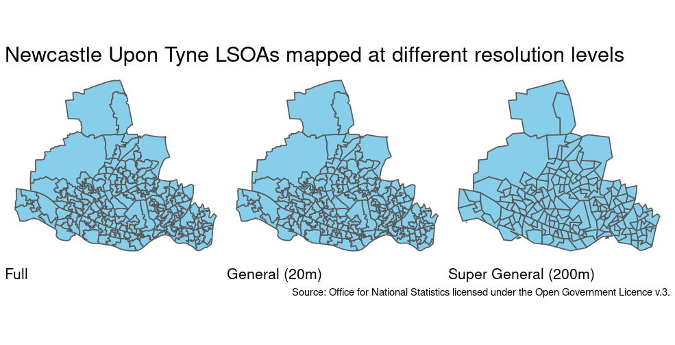
Before you even start playing with your data, ask yourself if you’ve got the appropriate data set for the job. Spatial data can come in different resolutions, and depending on the type of analysis or visualisation you are doing you might not need really accurate boundaries. Choosing a smaller file at the cost of a little accuracy can massively reduce the file size and read in times. Of course, you don’t always have the luxury of choosing your data, but if you can it can make a big difference.
For example, I live in the UK so I often use the Open Geography portal. This is hosted by the Office for National Statistics (ONS) and provides free and open access geographic data for the UK. The ONS provide boundaries for each geography at both full resolution and generalised formats that provide a smoothing of the full boundaries. The full resolution is the highest resolution data available, which can result in very large file sizes. Generalised formats preserve much of the original detail but are much smaller in size providing a good compromise.
For the types of visualisations I make, generalised data is sufficient.
As a small example, I downloaded the UK Lower layer Super Output Areas
datasets
with Full, Generalised and Super Generalised boundaries and calculated
the file sizes and time to read in. I also plotted the three different
resolutions with geom_sf() so you can compare how they look.
| Resolution | Generalised to | File size | Time to read |
|---|---|---|---|
| Full | 0m | 546 MB | 2s |
| Generalised | 20m | 50MB | 750ms |
| Super generalised | 200m | 16MB | 620ms |
File size and read times for various resolutions of the same data set.
The full resolution file is 10 times bigger than the generalised one, but visually it’s hard to see the difference between the boundaries. Remember that higher resolution data sets will also take longer to render when you plot them.
Read only what you need with SQL queries
Sometimes you only need a subset of the data you’ve been given. Let’s
say I have data for the UK, but I only need the LSOAs in Wales. It’s
inefficient to load the entire data set, to then immediately throw away
most of the rows. It would make much more sense for me to only load into
memory the rows that I need. In R, we use the st_read() function from
{sf} to parse spatial data. The query argument in st_read() allows
for reading just parts of the file into memory using SQL queries to
filter the data on disk.
The format of the query is SELECT columns FROM layer WHERE condition.
So to select all columns from my LSOA layer with code starting with “W”
(for Wales 🏴) we would use the following query.
library("sf")
st_read("data/Lower_layer_Super_Output_Areas_2021_EW_BGC_V3.gpkg",
        query = "SELECT * FROM LSOA_2021_EW_BGC_V3 WHERE LSOA21CD LIKE 'W%'",
        quiet = TRUE)
## Simple feature collection with 1917 features and 7 fields
## Geometry type: MULTIPOLYGON
## Dimension:     XY
## Bounding box:  xmin: 146615.2 ymin: 164586.3 xmax: 355312.8 ymax: 395982.3
## Projected CRS: OSGB36 / British National Grid
## First 10 features:
##     LSOA21CD              LSOA21NM  BNG_E  BNG_N     LONG      LAT
## 1  W01000003 Isle of Anglesey 001A 244606 393011 -4.33934 53.41098
## 2  W01000004 Isle of Anglesey 001B 242766 392434 -4.36671 53.40525
## 3  W01000005 Isle of Anglesey 005A 259172 377173 -4.11332 53.27280
## 4  W01000006 Isle of Anglesey 006A 240111 379172 -4.39991 53.28535
## 5  W01000007 Isle of Anglesey 009A 240423 370062 -4.39067 53.20362
## 6  W01000008 Isle of Anglesey 008A 253221 372359 -4.20027 53.22795
## 7  W01000009 Isle of Anglesey 007C 237013 376457 -4.44494 53.26002
## 8  W01000010 Isle of Anglesey 002A 250545 382806 -4.24524 53.32103
## 9  W01000011 Isle of Anglesey 008B 254994 372208 -4.17367 53.22708
## 10 W01000012 Isle of Anglesey 006B 246450 374976 -4.30288 53.24954
##                                  GlobalID                          SHAPE
## 1  {C18AD6F8-CD89-453E-A34A-B9ACE9B58203} MULTIPOLYGON (((244811.2 39...
## 2  {0ED47DC7-B1FE-4E63-84A6-995B701A39C0} MULTIPOLYGON (((241027.3 39...
## 3  {EA47EE1B-C4F6-442F-B2F3-58EEA678DB1E} MULTIPOLYGON (((259509.4 37...
## 4  {8FA5312C-C4CF-4B38-B7BD-44C824D15ED0} MULTIPOLYGON (((241039 3817...
## 5  {A6509D8B-7C3D-4260-BA0F-BCECFFBEEA66} MULTIPOLYGON (((245072.1 37...
## 6  {73F66A80-7EE7-4A98-899C-9702711DA427} MULTIPOLYGON (((253481.6 37...
## 7  {7AB711C3-C230-4236-877B-8746ED3E1DCA} MULTIPOLYGON (((235911.7 37...
## 8  {B5A77ECA-8CDC-4F82-B07E-3305622D1175} MULTIPOLYGON (((251300.9 38...
## 9  {F7037CC7-D94A-4B6B-BEDA-7F02CF2CC5A5} MULTIPOLYGON (((256049.2 37...
## 10 {A1A42AA3-FF44-4F13-9B60-82F9E7FB5681} MULTIPOLYGON (((246333.7 37...
Here * means SELECT all columns, and LIKE is used to match strings
against a pattern in the OGR SQL
dialect.
But what if you don’t know the names of the layer you want to read in?
You can use st_layers() to identify the layer(s) of interest without
reading in the entire data.
st_layers("data/Lower_layer_Super_Output_Areas_2021_EW_BGC_V3.gpkg")
## Driver: GPKG
## Available layers:
##            layer_name geometry_type features fields
## 1 LSOA_2021_EW_BGC_V3 Multi Polygon    35672      7
##                         crs_name
## 1 OSGB36 / British National Grid
But what if you don’t know the names of your columns? You can look at
the first polygon only to get an idea about the structure without
loading the entire data set. Just use the feature ID attribute to read
in just the first row of your data with WHERE FID = 1.
st_read("data/Lower_layer_Super_Output_Areas_2021_EW_BGC_V3.gpkg",
                     query = "SELECT * FROM LSOA_2021_EW_BGC_V3 WHERE FID = 1",
        quiet = TRUE)
## Simple feature collection with 1 feature and 7 fields
## Geometry type: MULTIPOLYGON
## Dimension:     XY
## Bounding box:  xmin: 531948.3 ymin: 181263.5 xmax: 532308.9 ymax: 182011.9
## Projected CRS: OSGB36 / British National Grid
##    LSOA21CD            LSOA21NM  BNG_E  BNG_N     LONG      LAT
## 1 E01000001 City of London 001A 532123 181632 -0.09714 51.51816
##                                 GlobalID                          SHAPE
## 1 {1A259A13-A525-4858-9CB0-E4952BA01AF6} MULTIPOLYGON (((532105.3 18...
This only reads in the top row of the data, which is an LSOA E01000001
in the City of London.
Spatial filtering
In the last example, we filtered our dataset before reading it into R by using some of the metadata that was attached to our spatial polygons. But what if you don’t have any columns that provide a useful filter? You can also filter by the spatial properties of your data. Let’s try and read in only the Welsh LSOAs again, but this time, using the spatial property only.
First we need to create a polygon that we want our LSOAs to overlap with. A boundary for Wales is available within the countries data set on Open GeoPortal.
library(dplyr)
library(ggplot2)

uk = st_read("data/Countries_December_2022_GB_BGC.gpkg")

wales = filter(uk, CTRY22NM == "Wales")
We then turn that geometry into a well-known text string. This is
simply a text representation of the polygon. We use st_geometry() to
grab the geometry column of the data frame, and then st_as_text() to
convert to a well-known text string.
wales_wkt =
  wales |>
  st_geometry() |>
  st_as_text()
This well-known text is just a string defining the outline of the polygon we want to use as our bounding box (here Wales). It looks a bit like this.
"MULTIPOLYGON (((313022.3 384930.5, 312931.3 385007.4, 312644.5 38519.8, ...)))"
We can then use that string in the wkt_filter argument of st_read()
to only read in LSOAs that overlap with the Wales polygon.
wales_lsoa =
  st_read("data/Lower_layer_Super_Output_Areas_2021_EW_BGC_V3.gpkg",
          wkt_filter = wales_wkt)
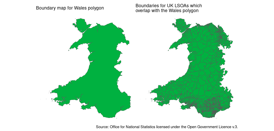
We can see that only the LSOAs that overlap with the polygon of Wales have been read in. Note that spatial intersection can be a little bit complicated. We’ve actually read in some English LSOAs along the Wales/England border in addition to the Welsh LSOAs because these technically overlap with the Wales polygon on the border itself. So it’s not perfect, but as a tool for selecting the rows of interest, before reading into R’s memory - it’s still pretty handy.
For another great example of using Spatial SQL to read in data efficiently, check out this nice blog post by Rob Williams.
Hopefully these quick tips will help you the next time you’re working with spatial data. If you want to learn more, check out our course on Spatial Data Analysis with R.