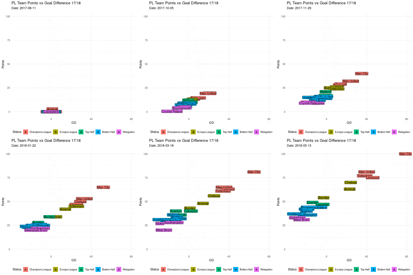
Animating the Premier League using {gganimate}

Ever wonder what an evolving gif of each premier league team’s goal difference vs points would look like made in R? Look no further! Most of this is going to be setting up the data (as always) instead of actually plotting the data. To get the data into shape, we’re going to be using the {tidyverse} and {lubridate}, which you can install the usual way via install.packages(). To animate the data we’ll be using the {gganimate} package. This is not on CRAN and so must be installed from GitHub, which you can do so via the {devtools} package
devtools::install_github("thomasp85/gganimate")
To get started let’s attach the relevant packages
library("tidyverse")
library("lubridate")
library("gganimate")
We’re going to use the last full season of matches in the premier league, which was the 17/18 season. The data was sourced from football-data.co.uk
prem = read_csv("http://www.football-data.co.uk/mmz4281/1718/E0.csv")
head(prem)
## # A tibble: 6 x 65
##   Div   Date  HomeTeam AwayTeam  FTHG  FTAG FTR    HTHG  HTAG HTR   Referee
##   <chr> <chr> <chr>    <chr>    <int> <int> <chr> <int> <int> <chr> <chr>
## 1 E0    11/0… Arsenal  Leicest…     4     3 H         2     2 D     M Dean
## 2 E0    12/0… Brighton Man City     0     2 A         0     0 D     M Oliv…
## 3 E0    12/0… Chelsea  Burnley      2     3 A         0     3 A     C Paws…
## 4 E0    12/0… Crystal… Hudders…     0     3 A         0     2 A     J Moss
## 5 E0    12/0… Everton  Stoke        1     0 H         1     0 H     N Swar…
## 6 E0    12/0… Southam… Swansea      0     0 D         0     0 D     M Jones
## # ... with 54 more variables
We’re only interested in the date, teams, result and home/away goals. These variables come between the variables Date and FTR. We also need to convert Date to a date object
prem = prem %>%
  select(Date:FTR) %>%
  mutate(Date = dmy(Date))
Cumulative points per day per team
There’s probably a better way to do this, but here is mine. I added a column for each team onto the data then, using a for loop (I know I’m sorry) I transferred the “H”, “A” and “D” status of the full time result into points for each time in their respective column. For you non-football heads, thats 3 for a win, 1 for a draw and 0 for a loss.
prem[sort(unique(prem$HomeTeam))] = NA

for(i in 1:nrow(prem)) {
  if(prem$FTR[i] == "H") {
    prem[i, prem$HomeTeam[i]] = 3
    prem[i, prem$AwayTeam[i]] = 0
  } else if(prem$FTR[i] == "A") {
    prem[i, prem$AwayTeam[i]] = 3
    prem[i, prem$HomeTeam[i]] = 0
  } else{
    prem[i, c(prem$AwayTeam[i], prem$HomeTeam[i])] = 1
  }
}
head(prem)
## # A tibble: 6 x 26
##   Date       HomeTeam AwayTeam  FTHG  FTAG FTR   Arsenal Bournemouth
##   <date>     <chr>    <chr>    <int> <int> <chr>   <dbl>       <dbl>
## 1 2017-08-11 Arsenal  Leicest…     4     3 H           3          NA
## 2 2017-08-12 Brighton Man City     0     2 A          NA          NA
## 3 2017-08-12 Chelsea  Burnley      2     3 A          NA          NA
## 4 2017-08-12 Crystal… Hudders…     0     3 A          NA          NA
## 5 2017-08-12 Everton  Stoke        1     0 H          NA          NA
## 6 2017-08-12 Southam… Swansea      0     0 D          NA          NA
## # ... with 18 more variables
You can see where Arsenal beat Leicester 4-3, there is a 3 in the Arsenal variable. Now, it would be nice to have this data in long form, for plotting purposes later, so we’ll use gather(). I then don’t want any rows with an NA in the Points variable, as these only occur if a team hasn’t played on that day.
prem_points = prem  %>%
  gather(Team, Points, Arsenal:`West Ham`) %>%
  select(Date, Team, Points) %>%
  drop_na(Points)
At the moment, we only have one row for each match on each day. Later, we’ll need to work out the position of each team on each day. To do this, we need the points for each team on each day, even if they didn’t play. So I’m going to create an empty data set of days and teams, join it then fill in the NA’s with 0’s.
empty = data.frame(Date = rep(unique(prem$Date), each = 20),
           Team = unique(prem$HomeTeam),
           stringsAsFactors = FALSE)
prem_points = left_join(empty, prem_points)

## Joining, by = c("Date", "Team")
prem_points[is.na(prem_points)] = 0
Now all we need to do is calculate the cumulative points for each team on each day over the course of the season
prem_points = prem_points %>%
  group_by(Team) %>%
  arrange(Date) %>%
  mutate(Points = cumsum(Points)) %>%
  ungroup()
So, for example, for Arsenal, the data now looks like this
prem_points %>%
  filter(Team == "Arsenal") %>%
  arrange(Date)
## # A tibble: 105 x 3
##    Date       Team    Points
##    <date>     <chr>    <dbl>
##  1 2017-08-11 Arsenal      3
##  2 2017-08-12 Arsenal      3
##  3 2017-08-13 Arsenal      3
##  4 2017-08-19 Arsenal      3
##  5 2017-08-20 Arsenal      3
##  6 2017-08-21 Arsenal      3
##  7 2017-08-26 Arsenal      3
##  8 2017-08-27 Arsenal      3
##  9 2017-09-09 Arsenal      6
## 10 2017-09-10 Arsenal      6
## # ... with 95 more rows
We have a row for each day there was a premier league match, even if that team didn’t play. Here you can see Arsenal won on the first day of the season (they beat Leicester 4-3) and gather any more points til the won again on the 9th of September.
Cumulative goal difference per team per day
We’re going to take the exact same process to do this job. Do let’s start by overwriting those columns of points in prem with columns of NA’s ready for the goal difference
prem[sort(unique(prem$HomeTeam))] = NA
Now, using a for loop again (again, I’m sorry) for each home team and away team we calculate the goal difference by simply minusing the away team goals from the home team goals or vice versa.
for(i in 1:nrow(prem)){
  prem[i, prem$HomeTeam[i]] = prem$FTHG[i] - prem$FTAG[i]
  prem[i, prem$AwayTeam[i]] = prem$FTAG[i] - prem$FTHG[i]
}
head(prem)
## # A tibble: 6 x 26
##   Date       HomeTeam AwayTeam  FTHG  FTAG FTR   Arsenal Bournemouth
##   <date>     <chr>    <chr>    <int> <int> <chr>   <int>       <int>
## 1 2017-08-11 Arsenal  Leicest…     4     3 H           1          NA
## 2 2017-08-12 Brighton Man City     0     2 A          NA          NA
## 3 2017-08-12 Chelsea  Burnley      2     3 A          NA          NA
## 4 2017-08-12 Crystal… Hudders…     0     3 A          NA          NA
## 5 2017-08-12 Everton  Stoke        1     0 H          NA          NA
## 6 2017-08-12 Southam… Swansea      0     0 D          NA          NA
## # ... with 18 more variables:
You can see now for when Arsenal beat Leicester 4-3, instead of having a 3 in the Arsenal variable, we have a 1 to signify Arsenal won by 1 goal. Now we follow the same process as before in that we gather the data into long format, join with the empty data set of days, turn the NAs into 0’s and then calculate the cumulative goal difference over the season.
prem_gd = prem  %>%
  gather(Team, GD, Arsenal:`West Ham`) %>%
  select(Date, Team, GD) %>%
  drop_na(GD)
prem_gd = left_join(empty, prem_gd)

## Joining, by = c("Date", "Team")
prem_gd[is.na(prem_gd)] = 0
prem_gd = prem_gd %>%
  group_by(Team) %>%
  arrange(Date) %>%
  mutate(GD = cumsum(GD)) %>%
  ungroup()
Now we need to join the two data sets!
prem_total = left_join(prem_points, prem_gd)
## Joining, by = c("Date", "Team")
Again using Arsenal as the example team, the data now looks like this
prem_total %>%
  filter(Team == "Arsenal") %>%
  arrange(Date)
## # A tibble: 105 x 4
##    Date       Team    Points    GD
##    <date>     <chr>    <dbl> <dbl>
##  1 2017-08-11 Arsenal      3     1
##  2 2017-08-12 Arsenal      3     1
##  3 2017-08-13 Arsenal      3     1
##  4 2017-08-19 Arsenal      3     0
##  5 2017-08-20 Arsenal      3     0
##  6 2017-08-21 Arsenal      3     0
##  7 2017-08-26 Arsenal      3     0
##  8 2017-08-27 Arsenal      3    -4
##  9 2017-09-09 Arsenal      6    -1
## 10 2017-09-10 Arsenal      6    -1
## # ... with 95 more rows
Now we can see not only when Arsenal picked up points, but when they dropped points as well. For example, on the 27th of August, they got beat by 4 goals as their goal difference shifted from 0 to -4.
We’re not done there! For the gif, we want to be able to display the current status of the team on each day i.e. Champions League (4th or above), Europa League (5th - 7th), Top Half (8th - 10th), Bottom Half (11th - 17th) or Relegation Zone (18th or below). To do this, on each day, we first need to retrieve the order of each team based on their points and goal difference
prem_total = prem_total %>%
  group_by(Date) %>%
  arrange(desc(Points), desc(GD)) %>%
  mutate(Position = row_number()) %>%
  ungroup()
After that, we can quite easily calculate their position status using our own function, and a bit of {purrr}
Qual = function(x){
  if(x <= 4){
    y = "Champions League"
  } else if(x <= 7){
    y = "Europa League"
  } else if(x <= 10){
    y = "Top Half"
  } else if(x <= 17){
    y = "Bottom Half"
  } else {
    y = "Relegation"
  }
  return(y)
}

prem_total = prem_total %>%
  mutate(Status = map_chr(Position, Qual),
         Status = factor(Status, levels = c("Champions League",
                                            "Europa League",
                                            "Top Half",
                                            "Bottom Half",
                                            "Relegation")))
head(prem_total)
## # A tibble: 6 x 6
##   Date       Team     Points    GD Position Status
##   <date>     <chr>     <dbl> <dbl>    <int> <fct>
## 1 2018-05-13 Man City    100    79        1 Champions League
## 2 2018-05-09 Man City     97    78        1 Champions League
## 3 2018-05-10 Man City     97    78        1 Champions League
## 4 2018-05-06 Man City     94    76        1 Champions League
## 5 2018-05-08 Man City     94    76        1 Champions League
## 6 2018-04-29 Man City     93    76        1 Champions League
Note that here I’m using a factor to reorganise the legend in the plot we’re about to make. We’re looking for a path of a teams points and goal difference over a season, with a colour scheme for where they are in the table at that point. This is what that looks for one team (here I’m using Newcastle United)
 prem_total %>%
    filter(Team == "Newcastle") %>%
    arrange(Date) %>%
    ggplot(aes(GD, Points)) +
    geom_point(aes(colour = Status), size = 3) +
    geom_path(linetype = 2, alpha = 0.4) +
    theme_minimal() +
    labs(title = "NUFC Points/Goal Difference Path",
         subtitle = "Season 2017/2018") +
    theme(legend.position="bottom") +
    scale_colour_brewer(type = "qual",
                        palette = "Paired")

Bear in mind we’re going to have 20 teams on the graph and so instead of just using points, we’re going to use labels with the team’s name on.
Now, adding {gganimate} is relatively pain-free. The package comes with lots of functions titled transition_*(). These dictate by what variable your gif will change. We want our gif to be over time i.e. the variable Date. There is a specific transition function that works with time, called transition_time(). {gganimate} is also lovely in the way that we can just add these functions to regular ggplots.
g = prem_total %>%
  arrange(Date) %>%
  ggplot(aes(GD, Points)) +
  geom_label(aes(label = Team, fill = Status), label.padding = unit(0.1, "lines")) +
  theme_minimal() +
  labs(title = "PL Team Points vs Goal Difference 17/18",
  subtitle =  "Date: {frame_time}") +
  scale_colour_brewer(type = "qual",
  palette = "Paired") +
  theme(legend.position = "bottom") +
  transition_time(Date)

animate(g, nframes = 200, fps = 2)

We’ve only added one function here. Easy! If you are wanting to split it up by something more arbitrary (a character variable let’s say), then you would use transition_states(). Then all that is needed is the animate function! Within the animate() function, the nframes argument is the total number of frames whilst the fps argument is the total number of frames per second. If we wanted our gif to be a bit quicker, we’d go for a higher frame per second.
That’s all for now, thanks for reading!

