Vetiver: MLOps for Python
This post is the fourth in our series on MLOps with vetiver:
- Part 1: Vetiver: First steps in MLOps
- Part 2: Vetiver: Model Deployment
- Part 3: Vetiver: Monitoring Models in Production
- Part 4: Vetiver: MLOps for Python (this post)
Parts 1 to 3 introduced the {vetiver} package for R and outlined its far-reaching applications in MLOps. But did you know that this package is also available in Python? In this post we will provide a brief outline to getting your Python models into production using vetiver for Python.
Installation
Like any other Python package on PyPI, vetiver can be installed using pip. Let’s set up a virtual environment and install all of the packages that will be covered in this blog:
python -m venv venv/
source venv/bin/activate
pip install vetiver pandas pyjanitor scikit-learn pins
Check out our previous blog about virtual environments in Python for more details.
Data
We will be working with the World Health Organisation Life Expectancy data which provides the annual average life expectancy in a number of countries. This can be downloaded from Kaggle:
import pandas as pd

url = "https://www.kaggle.com/api/v1/datasets/download/kumarajarshi/life-expectancy-who"
data = pd.read_csv(url, compression = "zip")
data.head()
#>        Country  Year  ... Income composition of resources  Schooling
#> 0  Afghanistan  2015  ...                           0.479       10.1
#> 1  Afghanistan  2014  ...                           0.476       10.0
#> 2  Afghanistan  2013  ...                           0.470        9.9
#> 3  Afghanistan  2012  ...                           0.463        9.8
#> 4  Afghanistan  2011  ...                           0.454        9.5
#>
#> [5 rows x 22 columns]
Let’s drop missing data, clean up the column names and select a subset of the variables to work with:
import janitor

data = data.dropna()
data = data.clean_names(strip_underscores=True)
data = data[[
    "life_expectancy",
    "percentage_expenditure",
    "total_expenditure",
    "population",
    "bmi",
    "schooling",
]]
data.head()
#>    life_expectancy  percentage_expenditure  ...   bmi  schooling
#> 0             65.0               71.279624  ...  19.1       10.1
#> 1             59.9               73.523582  ...  18.6       10.0
#> 2             59.9               73.219243  ...  18.1        9.9
#> 3             59.5               78.184215  ...  17.6        9.8
#> 4             59.2                7.097109  ...  17.2        9.5
#>
#> [5 rows x 6 columns]
Vetiver is compatible with models built in scikit-learn, PyTorch, XGBoost and statsmodels. The actual modelling process is not so important in this blog. We will be more interested in how we go about taking this model into production using vetiver. So let’s go with a simple K-Nearest Neighbour model built using scikit-learn:
from sklearn.neighbors import KNeighborsRegressor
from sklearn.pipeline import Pipeline
from sklearn.preprocessing import StandardScaler

target = "life_expectancy"
covariates = [
    "percentage_expenditure",
    "total_expenditure",
    "population",
    "bmi",
    "schooling",
]
y = data[target]
X = data[covariates]

model = Pipeline(
    [
        ("transform", StandardScaler()),
        ("model", KNeighborsRegressor()),
    ]
)
model.fit(X, y)
#> Pipeline(steps=[('transform', StandardScaler()),
#>                 ('model', KNeighborsRegressor())])
Let’s break down what’s happened here:
- We selected our target variable (life expectancy) and the covariates (features) that will be used to predict the target.
- We constructed a modelling pipeline which includes:
- Preprocessing of input data via standardisation.
- K-Nearest Neighbours regression.
- In the final step, we fitted our model to the training data.
Usually at this point we would evaluate how our model performs on some unseen test data. However, for brevity we’ll now go straight to the MLOps steps.
MLOps
In a typical MLOps workflow, we are setting up a continuous cycle in which our trained model is deployed to a cloud environment, monitored in this environment, and then retrained on the latest data. The cycle repeats so that we are always maintaining a high model performance and avoiding the dreaded model drift (more on this later).
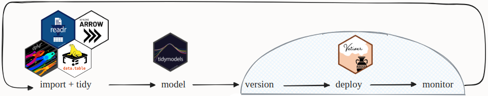
From the diagram above, the crucial steps that set this workflow apart from a typical data science project are model versioning, deployment and monitoring. We will go through each of these in turn using vetiver.
Before we can begin, we must convert our scikit-learn model into a “vetiver model”:
import vetiver

v_model = vetiver.VetiverModel(model, model_name="KNN", prototype_data=X)
print(type(v_model))
#> <class 'vetiver.vetiver_model.VetiverModel'>
print(v_model.description)
#> A scikit-learn Pipeline model
print(v_model.metadata)
#> VetiverMeta(user={}, version=None, url=None, required_pkgs=['scikit-learn'], python_version=(3, 10, 12, 'final', 0))
Our VetiverModel object contains model metadata and dependencies
(including the Python packages used to train it and the current Python
version). The model_name will be used to identify the model later on,
and the prototype_data will provide some example data for the model
API (more on this below).
Model versioning
In a cycle where our model is continuously being retrained, it is important to ensure that we can retrieve any models that have previously been deployed. Vetiver utilises the pins package for model storage. A pin is simply a Python object (could be a variable, data frame, function, …) which can be stored and retrieved at a later time. Pins are stored in “pins boards”. Examples include:
- Local storage on your device
- Google Drive
- Amazon S3
- Posit Connect
Let’s set up a temporary pins board locally for storing our model:
from pins import board_temp

model_board = board_temp(
    versioned=True, allow_pickle_read=True
)
vetiver.vetiver_pin_write(model_board, v_model)
#> Model Cards provide a framework for transparent, responsible reporting.
#>  Use the vetiver `.qmd` Quarto template as a place to start,
#>  with vetiver.model_card()
#> Writing pin:
#> Name: 'KNN'
#> Version: 20250220T141808Z-af3d5
Enabling allow_pickle_read will allow quick reloading of the model
later on, whenever we need it.
At this stage our VetiverModel object is now stored as a pin, and we
can view the full list of “KNN” model versions using:
model_board.pin_versions("KNN")
#>               created   hash                 version
#> 0 2025-02-20 14:18:08  af3d5  20250220T141808Z-af3d5
As expected, we only have one version stored so far!
Model deployment
If we want to share our model with other users (colleagues, stakeholders, customers) we should deploy it to an endpoint on the cloud where it can be easily shared. To keep things simple for this blog, and to ensure the code examples provided here are fully reproducible, we will just deploy our model to the localhost.
First we have to construct a model API. This is a simple interface which takes some input and gives us back some model predictions. Crucially, APIs can be hosted on the cloud where they can receive input data via HTTP requests.
Our VetiverModel object already contains all of the info necessary to
build an API using the FastAPI
framework:
app = vetiver.VetiverAPI(v_model, check_prototype=True)
Running app.run(port=8080) will start a local server for the model API
on port 8080. We are then presented with a simple graphical interface in
which we can run basic queries and generate predictions using our model.
The prototype_data argument which we defined when constructing our
VetiverModel (see above) is used here to provide some example input
data for queries:
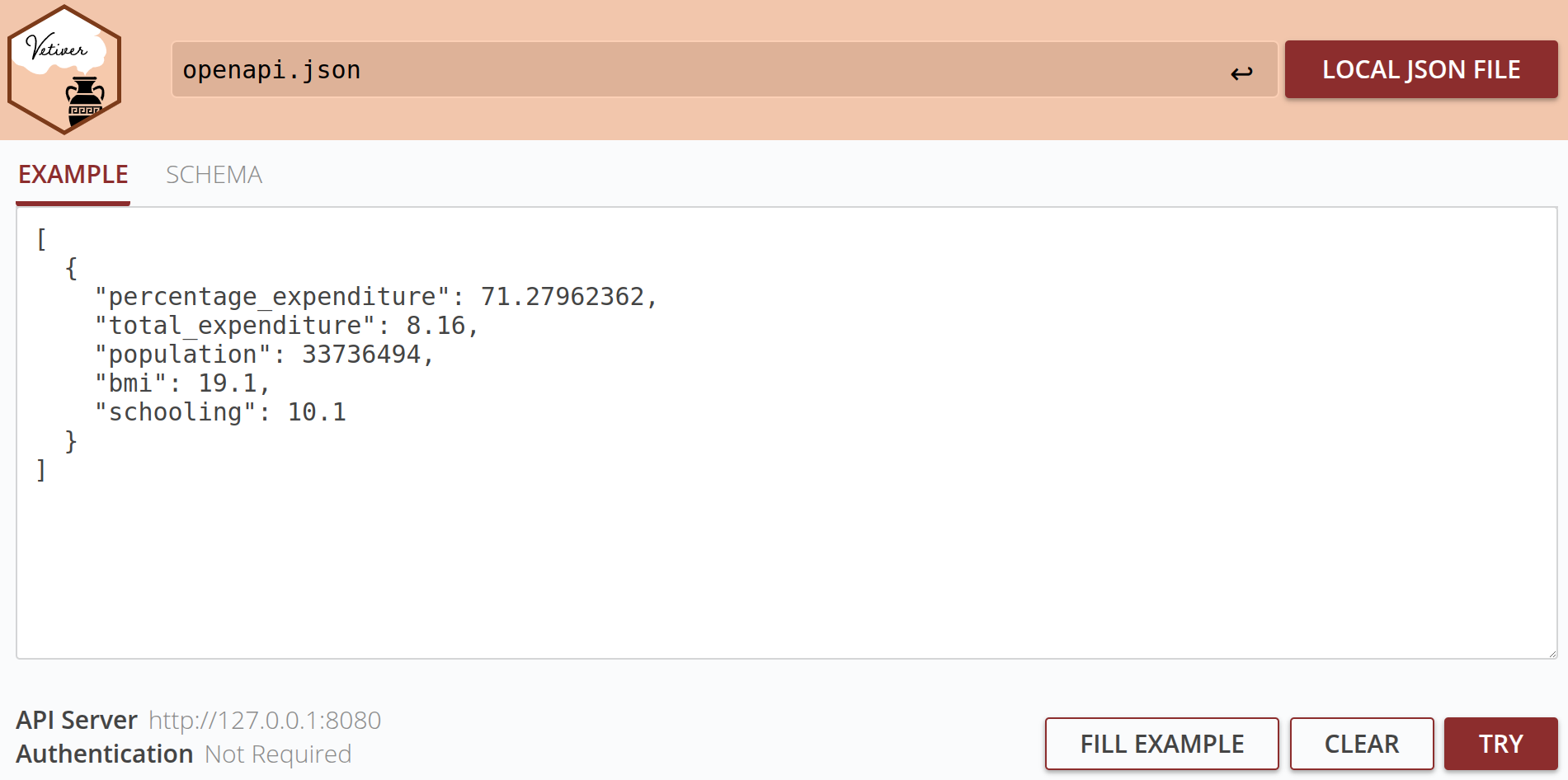
Alternatively we can also submit queries from the command line. The
graphical interface above provides template curl commands which can be
copied into the command line and executed against the model. For
example, the input data shown in the above screenshot can be fed into
the model via a POST request:
curl -X POST "http://127.0.0.1:8080/predict" \
 -H "Accept: application/json" \
 -H "Content-Type: application/json" \
 -d '[{"percentage_expenditure":71.27962362,"total_expenditure":8.16,"population":33736494,"bmi":19.1,"schooling":10.1}]' \
The same command would work for querying APIs on the cloud as long as the IP address for the API endpoint (here it is http://127.0.0.1, which points to the localhost) is updated accordingly.
Deploying your model locally is a great way to test that your API behaves as you expect. What’s more, it’s free and does not require setting up an account with a cloud provider! But how would we go about deploying our model to the cloud?
If you already have a server on Posit
Connect, it’s just a
case of running vetiver.deploy_rsconnect() (see the Posit vetiver
documentation for
more details). If you don’t have Posit Connect, not to worry! Instead
you can start by running:
vetiver.prepare_docker(model_board, "KNN")
This command is doing a lot of heavy lifting behind the scenes:
- Lists the Python package dependencies in a vetiver_requirements.txt file.
- Stores the Python code for the model API in an app.py file.
- Creates a Dockerfile containing the Python version requirement for the model and the docker commands for building and running the API. An example is shown below:
# # Generated by the vetiver package; edit with care
# start with python base image
FROM python:3.10

# create directory in container for vetiver files
WORKDIR /vetiver

# copy  and install requirements
COPY vetiver_requirements.txt /vetiver/requirements.txt

#
RUN pip install --no-cache-dir --upgrade -r /vetiver/requirements.txt

# copy app file
COPY app.py /vetiver/app/app.py

# expose port
EXPOSE 8080

# run vetiver API
CMD ["uvicorn", "app.app:api", "--host", "0.0.0.0", "--port", "8080"]
With these files uploaded to the cloud server of your choosing, the
docker build command will take care of the rest. This process can be
automated on AWS, Google Cloud Run, Azure, and many other cloud
platforms.
Model monitoring
Success! Your model is now deployed and your users are interacting with it. But this is only the beginning…
Data changes! Over time you will notice various aspects of your data changing in unexpected ways:
- The way the data is distributed may change (data drift).
- The relationship between the target variable and covariates may change (concept drift).
These two processes will conspire to create model drift, where your model predictions start to drift away from the true values. This is why MLOps is not simply a one-off deployment. It is a continuous cycle in which you will be retraining your model on the latest data on a regular basis.
While we will not be providing a full worked example of model drift here, we will just mention some helpful functions provided by vetiver to deal with this problem:
vetiver.compute_metrics(): computes keys metrics at specified time intervals, allowing us to understand how the model performance varies over time.vetiver.pin_metrics(): stores the model metrics in a pins board for future retrieval.vetiver.plot_metrics(): plots the metrics over time.
You can get an idea of how these Python methods can be used by reading our previous blog post where we monitored the model’s performance using vetiver for R.
The metrics can be entirely defined by the user, and might include the
accuracy score for a classification model and the mean squared error for
a regression model. We can also make use of predefined scoring functions
from the sklearn.metrics library.
For more on model monitoring, check out the Posit vetiver documentation.
Summary
Hopefully by reading this post you will have a better understanding of MLOps and how to get started with MLOps in Python. Most importantly, you don’t have to be an expert in AWS or Azure to get started! Vetiver provides intuitive, easy-to-use functions for learning the crucial steps of MLOps including versioning your model, building a model API, and deploying your model using docker or Posit Connect.
For some further reading, check out:
- Our previous blog posts on vetiver with R.
- The Posit vetiver documentation.